
Time to Send a Signal
In the last chapter we learned about how RF travels. Today we learn about what components we need to have for RF to be transmitted and received and how they are measured. We will also learn about the math behind it and how to calculate it quickly. Please take your seats class!
RF Components
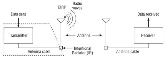
Let’s start at the beginning. So you have a signal and you want to send that across the building to another station. How does it get there from an RF perspective? The first thing that will need to happen is for the signal to hit your Transmitter. The transmitter is the initial component in the creation of the wireless medium. Its job is to take the data provided and modify it using a modulation technique like the ones we went over in Chapter 1. It is then turned into a carrier signal. You may have heard the term transceiver, which is just a way to say that the radio can transmit and receive at the same time. After the signal has been converted into the carrier signal it is sent to the Antenna which collects the AC signal from the transmitter and directs or radiates the RF wave away from the antenna in a specific pattern dictated by the antenna type, which then is directed toward the receiver. On the receiving end, the signal would arrive via another antenna and then on to the Receiver. The receiver takes the carrier signal and demodulates it back into 1’s and 0’s, passing it on the the station. It is important to note that the receiver is taking in a signal that has been affected by distance, free space path loss, as well as many of the items discussed in Chapter 3, such as absorption. The diagram below is a great representation of how this looks. We will be going over Intentional Radiator and EIRP in the next section.
Let’s Go to the Isotropics
As the signal travels from the transmitter to the antenna, there are a few items of note we need to pay attention to. We need to pay attention to them because they are both regulated by the FCC and breaking laws are bad!

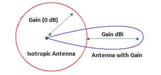
First let’s talk about the Isotropic Radiator, which is a point source that radiates in all directions. In the CWNA book, this is compared to the sun, which radiates energy equally in all directions. This will become important later when we discuss dBi (decibels relative to an isotropic radiator). Next we need to talk about the Intentional Radiator. The intentional radiator is defined as something that has the sole purpose of generating RF. The power generated is regulated by the FCC as we have mentioned before. An IR consists of everything from the transmitter to the end of the connector that attaches to the antenna, but not including the antenna. This includes the cable, connectors, arrestors, and transmitter. IR is measured in mW or dBm. Once we pass the IR we get to EIRP (Equivalent Isotropically Radiated Power) which is the highest output of RF signal leaving the antenna. Antennas by nature are designed to focus the RF, which then increases the amplitude of the signal. Again, this is FCC regulated.
Time for a New Unit
Units of Power and Comparison that is. Units of power are considered absolute, meaning it is actual. If we said that a road is a mile long, that would be an absolute measurement. If we were using unit of comparison, we would say this road is 1/2 as long as that road.
Units of Power (absolute):
- watt (W)
- milliwatt (mW)
- decibels relative to 1 mW (dBm)

Units of Comparison (relative):
- decibel (dB)
- decibels relative to an isotropic radiator (dBi)
- decibels relative to a half-wave dipole antenna (dBd)
Watt: equal to 1 amp of current flowing at 1 volt, also equal to volts x amps
Milliwatt: 1/1000 of a watt, most 802.11 devices transmit between 1 mW and 100 mW
Decibel: a decibel is a unit of comparison which measures the change in power. It is derived from bel which is equal to a 10:1 ratio. A decibel is 1/10 of a bel.
Decibels relative to an Isotropic Radiator (dBi): this is the gain, or increase in power over what an isotropic radiator would generate. It is the measurement of antenna gain, measured at the strongest point of the antenna. A half-wave dipole antenna is 2.14dBi.
Decibels relative to a half-wave dipole antenna (dBd): dBd is the gain, or increase of an antenna relative to a dipole antenna. dBd is onmidirectional antenna gain.
Decibels relative to 1 mW (dBm): this is an absolute assessment that measures a change in power referenced to 1 mW. 0 dBm = 1 mW. It is important to know that a +6dB signal doubles the distance of a usable signal and a -6dB signal halves the usable distance.
Watts going on
I’m sorry, I couldn’t help it. My girls in the other room doing homework surely just rolled their eyes at me. But as a dad, I consider it my duty to make dad jokes. Moving on….. When I first saw that I had to learn RF Math I assumed this was going to be like learning subnetting for the first time. Thankfully this is infinitely more easy to understand. So what makes up RF Math?
Rules of 10’s and 3’s
It is important to remember that this is not exact math we are doing here. There are formulas for when you need exact numbers, but this is provided to allow for close approximation.
- For every 3dB of gain (relative) double the absolute power (mW)
- For every 3dB of loss (relative) halve the absolute power (mW)
- For every 10dB of gain (relative) multiply the absolute power (mW) by a factor of 10
- For every 10 dB of loss (relative) divide the absolute power (mW) by a factor of 10
Let’s go over a quick example:You have a signal with an output of 25mW attached to a cable that has -6dB of loss that attaches to an antenna with 3dBi of gain. Since we know that 0 dBm is equal to 1 mW, we will start there. So to get to 25mW we first multiply 1mW x 10 which we would then need to then add 10dBm, we aren’t at 25mW yet so we keep going. We can’t multiply by ten again as that would put us over so this time we will double it, bringing us to 20mW. Since we doubled we would add 3 dBM to the 10 we already had giving us 13dBm which is pretty close. Had we done the actual math we would get 13.9794dBm. We can’t get any closer than that using 10’s and 3’s so let’s stay there and work with the rest of the equation. We now need to subtract the cable loss from our 13dBm so we subtract -6dBm giving us 7dBm. The last thing we need to do is add the antenna gain of 3dBi giving us a total output of 10dBm or 10mW. This is an example of why you need to have a Link Budget, which is the sum of all planned and expected gains and losses from the transmitting radio, through the RF medium to the receiver. Update to above example:It has been brought to my attention, that while my math is correct above, I could have been much more exact instead of close….see comments at the bottom. I wanted to leave the above example there instead of editing it so you can see the error I made and how to correct it. I learn the most from mistakes I make and hopefully you will as well. So for the original signal above, which was 25mW, we could have done something I should have shown you but neglected to remember at the time of writing. You can always go beyond your target output and work your way back. So to get to 25mW, we could have first multiplied 1 x 10 (10mW) +10dBm, then by 10 again (100mW) +10dBm, now 20dBm, divide by 2 (50mW) -3dBm now 17dBm, divide by 2 again (25mW) -3dBm arriving finally at 14dBm. We would then take the difference between the cable loss and antenna gain and subtract the last 3dBm to get 11dBm. If we wanted to convert 11dBm back to milliwatt, we could do on the dBm side +10,+10,-3,-3,-3 to get to 11 which on the mW side would be x10=10, x10=100, /2=50, /2=25, to the final of /2=12.5mW.
Check out this great explanation from Jerome Henry
What’s that Noise
In every environment you will have noise, which you will need to overcome to get your signal heard. The Noise Floor is the ambient or background level of radio energy on a specific channel. Anything electromagnetic has the potential of raising the amplitude of the noise floor on a specific channel. We measure this with SNR (Signal to Noise Ratio). SNR is the difference between the noise floor and the received signal, so if your RSSI (get to that in a second) is -50dBm and the noise floor is -80dBm then the SNR is 30dB, the difference between the two. An SNR of 25dB is considered good. Additionally we have SINR (Signal to Interference plus Noise Ratio). This is similar to SNR but is defined as the difference between the power of the primary RF signal, compared against the sum of power of the RF interference and background noise. The key here is the addition of interference which makes this a better indicator of what is happening at a specific time. The last two items we need to discuss are RSSI (Received Signal Strength Indicator) and Fade Margin. RSSI is the relative metric used by 802.11 radios to measure signal strength and is normally measured in dBm. Fade margin is the level of signal above what is required. The higher the fade margin the more reliable the link.
End of Chapter Review
In this chapter we learned some very important items. We now understand what makes up the components that help send an RF signal. We know how the signal is measured as well as how we can calculate our output given the entire RF component chain. And lastly we understand how noise has an effect on signal strength. I think one of the most important parts of this chapter is being able to take the power of 10’s and 3’s and quickly in your head (for most equations) figure out your rough RF signal output in the field while doing design. It will also be helpful to make sure you aren’t breaking any local laws by calculating those outputs in advance. As always please share using the links below, follow me and subscribe to the newsletter, and I’m off to study Chapter 5!


Good work.
Tomorrow next chapter.
Thanks a lot
I’m hoping to start Chapter 5 tonight, maybe get the post out Sunday night or Monday. Gotta balance family time in here!
Of cause you can get to 25mW with 10s and 3s.
To get exact to 25 mW instead of accepting 20mW as close enough.
Calculate the source.
Start with 100mW = 20 dBm (10*10)=10+10
Divide 100 in half two times which gets you to 50 and then 25. So subtract 3 two times on the dB side. 20-3-3=14 dBm. 25mW eq 14dBm
Then for the link:
Combine the -6dB and +3dB on the link to -3dB. Substract 3 from 14dBm (25mW) to get 11 dBm which is the correct result on the dBm side. Not 10 as in your example. Convert 11 dBm to mW by taking 100mW and divide in half 3 times (-3-3-3 in the dB world), which then equals 12,5 mW.
Your completely right. I totally missed that. I am going to edit the post but leave the original math I did showing how you can make a mistake like I did. Good find, thank you!
Nice blog Mike!
Might be an easier to digest example for SNR to use a noise level lower than the actual RSSI. So instead of -20dBm, use -80dBm since we typically want the signal higher than the noise floor.
Just my .02, keep it up!
-Keith
Good catch, it was not supposed to be -20….typo, and fixed.